webPIPSA

Protein Interaction Property Similarity Analysis

• Home
• Run PIPSA
• Documentation
• Demonstration
• Download
• References
• Funding
• Project
  Information
• Imprint
  Privacy
• Terms and Conditions

Part 2: Relating kinetic parameters to PIPSA results

This dataset consists of the modelled structures of Triosephosphate isomerases (TPI) from different species as described in the following publication:

qPIPSA: Relating enzymatic kinetic parameters and interaction fields. Razif R Gabdoulline, Matthias Stein and Rebecca C Wade BMC Bioinformatics 2007, 8:373 (fulltext)

To follow this example you should firstly run the demonstration Part 1.

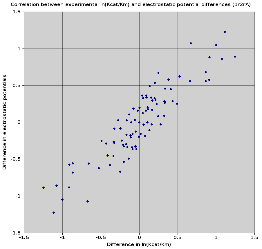
Plot the correlation between experimental ln(Kcat/Km) values and the electrostatic potential differences for TPI the x- and y- values are needed. Whereas the y-values are the differences in the electrostatic potentials and the x-values are the differences in ln(Kcat/Km).

After completing the PIPSA run of Part 1 of the demonstration, you will find some *.log files in the job directory (see the email notification that you recieved after submitting the job).

Since in this example, 2 regions are specified:

• 1.068, 4.059, 21.111, 15 (binding site)
• 8.15, 3.54, 34.83, 15 (catalytic loop)

you will find 3 *.log files:

• simsbindingsite.log
• simscatalyticloop.log
• sims.log

which, respectively, contain the comparison for the two specified regions and for the whole protein.
The files contain a column with the differences in electrostatical potentials between all the proteins, which are used as the y-values in the plot (see the publication above for further details).

To extract the pertinent column out of the *.log files (e.g. sims.log) you can

1. either import the files in OpenOffice/Excel. The corresponding values are then in the N-column of the Spreadsheet.
2. Or you could also use the linux command:
   cat sims.log | grep -v addH | cut -c126-139

In the paper above, the Km and Kcat values were retrieved from BRENDA and SABIO-RK. The complete list is available here. Since creating the difference for each y-value would be very time-consuming and error-prone, this script automates the procedure.
Running the command:

perl createPlot.pl sims.log kineticDataTable.txt > sims.plot

The kineticDataTable.txt should contain 2 coulums. The first is the kinetic value and the second is the name of the corresponding protein file (without addH). Also every protein of the sims*.log should be listed in this table in the same order.
The created plot-file can then be plotted either gnuplot, OpenOffice, Excel, xmgrace or any other plotting tool you are familiar with.

In this demonstration the template used was the crystal structure 1R2RA. The correlation can alter depending on the template used to create the protein models. In Part 3 several templates have been used to examine the differences resulting from structural variations.